S-JEPA: A Stochastic Latent Variable Generalization of
Joint-Embedding Predictive Architectures

Overview

TL;DR

S-JEPA replaces the deterministic auxiliary token \(z\) in JEPAs with a proper stochastic latent variable, trained as a CVAE entirely in representation space, with no decoders and no reconstruction. The result: stronger representations than I-JEPA under matched architectures and schedules, plus error-correlated predictive uncertainty and diverse completions, capabilities no deterministic JEPA predictor has.

Abstract

The JEPA blueprint. In I-JEPA,
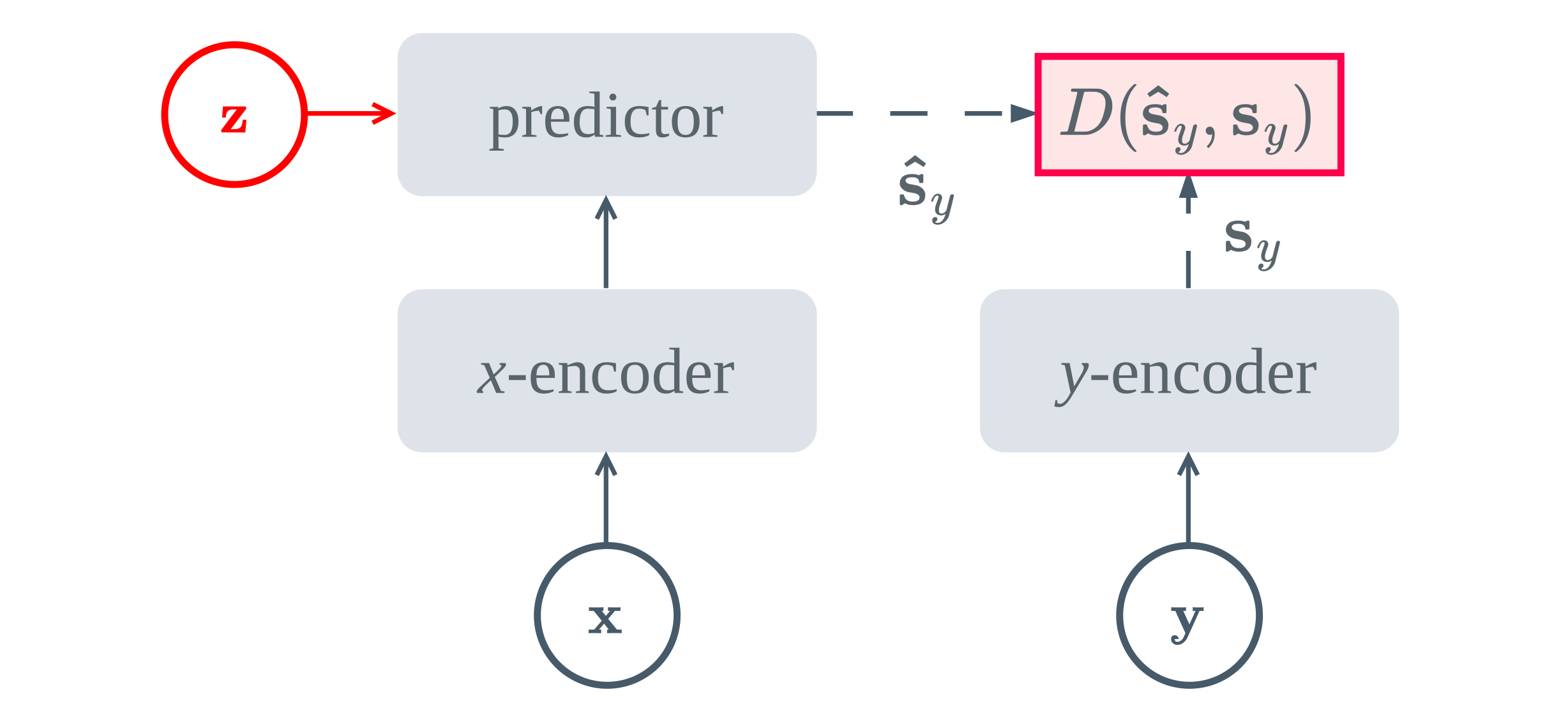
\(z\) is a fixed, deterministic token

S-JEPA overview. In S-JEPA, \(z\) is a stochastic
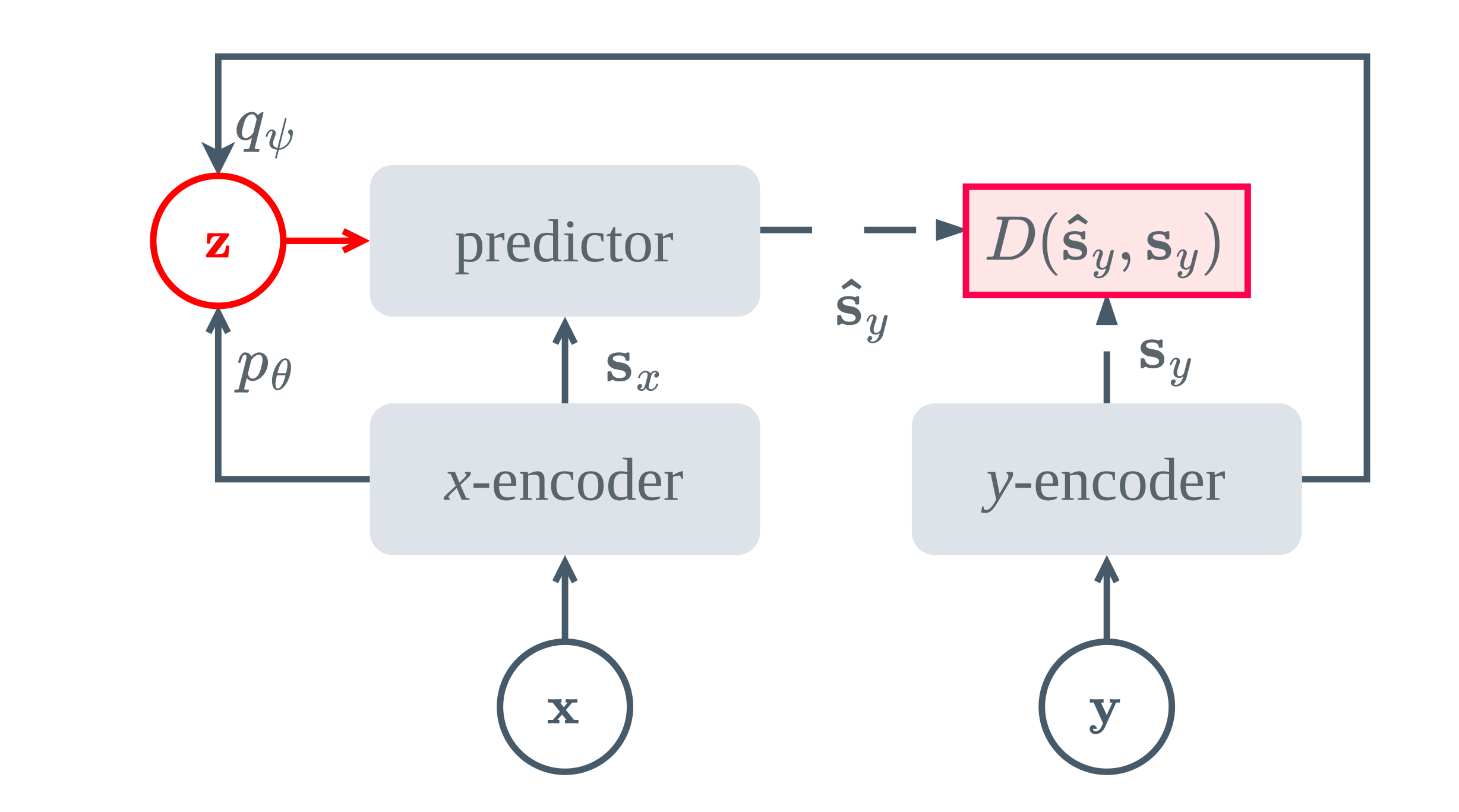
latent variable with a learned prior and posterior

Motivation

Why should prediction be stochastic?

A JEPA comprises a context encoder \(f_x\), a target encoder \(f_y\), and a predictor \(g\) that estimates \(\hat{s}_y = g(s_x, z)\) from the context representation \(s_x = f_x(x)\) and an auxiliary variable \(z\). In LeCun's original blueprint, \(z\) is meant to carry the residual information the context lacks: scene-level factors, global style, or the semantic content of a masked region. Yet in every instantiation to date, from I-JEPA's shared learnable mask token to V-JEPA's spatiotemporal analogue, \(z\) is deterministic. Stochasticity has only ever entered the positional component (where to mask), never the content of what is masked.

Our approach

We realise \(z\) as a proper stochastic latent variable over the content of the masked region, replacing the deterministic predictor with one built on a Conditional Variational Autoencoder (CVAE) operating entirely in representation space, i.e., with no pixel decoder and no reconstruction loss. A learned posterior infers \(z\) from context and target during training; a learned context-conditioned prior anticipates plausible completions from context alone and is used at inference.

Method

From a deterministic predictor to a CVAE in representation space

The I-JEPA objective

A JEPA computes \(s_x = f_x(x)\), \(s_y = f_y(y)\), and \(\hat{s}_y = g(s_x, z)\), and is trained to regress the target representation under a stop-gradient on the (EMA) target encoder:

A latent-variable model over target representations

We instead model the conditional distribution \(p(s_y \mid s_x)\) directly. We introduce \(z \in \mathbb{R}^{d_z}\) as a per-image latent variable that accounts for residual uncertainty, i.e., occlusion, texture variability, and semantic ambiguity, giving the joint and marginal:

Context-conditioned prior & approximate posterior

The prior sees the context \(s_x\) only, and must learn to anticipate plausible completions without the target. The posterior additionally sees the target \(s_y\) during training, inferring the \(z\) that best explains it. Both are diagonal Gaussians:

Evidence lower bound

Introducing the posterior and applying Jensen's inequality to the concave log yields the CVAE ELBO, in representation space:

Gaussian likelihood ⇒ squared error

Assuming a fixed-variance isotropic Gaussian likelihood around the predictor's output, the expected log-likelihood reduces in closed form to a scaled MSE:

The S-JEPA objective

Absorbing the constant \(1/(2\sigma^2)\) into a free hyperparameter \(\beta > 0\) that controls the information bottleneck on \(z\) gives the final training objective:

What this enables at inference

Results

Stronger representations, at matched compute

Under matched architectures and training schedules, S-JEPA improves over the deterministic I-JEPA baseline on linear evaluation and low-shot ImageNet-1K, and exceeds LeJEPA at matched architecture on a longer schedule, all with only \(1.01\times\) the parameters of I-JEPA and negligible overhead in FLOPs and inference latency.

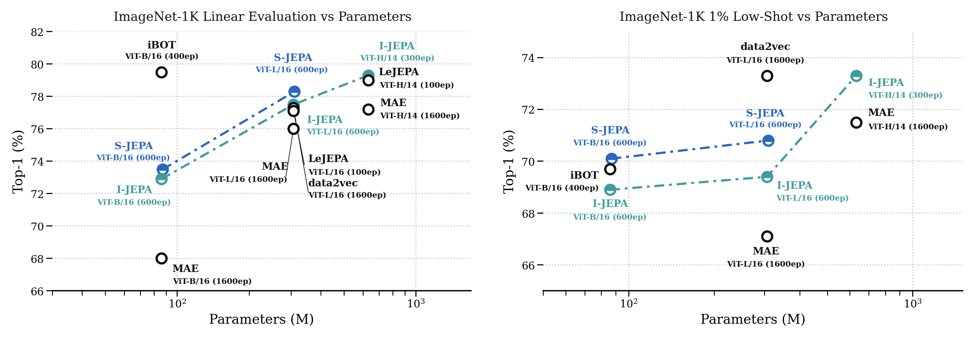
S-JEPA (blue) consistently sits above the I-JEPA / LeJEPA frontier (teal) at matched parameter count, on both linear evaluation (left) and 1% low-shot transfer (right) on ImageNet-1K. At ViT-L/16 (600 epochs), S-JEPA reaches 78.3% linear top-1, above I-JEPA (77.5%) and data2vec (77.3%, 1600 epochs); at ViT-B/16, S-JEPA reaches 73.5%, above I-JEPA (72.9%) and MAE (68.0%, 1600 epochs).

Representation structure

PCA projections of encoder features

We project block-4 patch representations onto their first three principal components (foreground-masked, mapped to RGB) across three ViT-B/16 encoders trained with different objectives. No localisation signal supervises this map, so the structure emerges purely from the pretraining objective. Select an example:

All three methods recover coherent object/background structure, with S-JEPA exhibiting particularly clear object boundaries and spatially consistent representations, suggesting that stochastic prediction preserves, and potentially sharpens, the semantic structure of the learned features.

Predictive uncertainty

Error-correlated uncertainty maps

For S-JEPA we draw \(N=50\) samples \(z \sim p_\theta(z\mid s_x)\) from the full-image context and compute the predictive variance \(U_p\) across the resulting target predictions. I-JEPA's deterministic predictor gives \(U_p = 0\) everywhere by construction, so its column below carries no information about the image, reflecting only the colour-map normalisation. S-JEPA's uncertainty, by contrast, consistently concentrates on the animal or object rather than the background, and correlates with where its own mean prediction actually errs. Select an example:

Diverse completions

Sampling the masked region

Each example shows a masked input and five completions, each from a distinct draw \(z_i \sim p_\theta(z\mid s_x)\), decoded via a lightweight diffusion decoder (RCDM) trained on frozen S-JEPA predictor representations. Decoding uses a fixed noise seed across all five draws, so the pixel-level variation you see reflects only the sampled latent, not decoder-side stochasticity. Select an example:

Samples vary in object identity and configuration, reflecting genuine uncertainty over the masked region encoded in \(z\), a capability the deterministic I-JEPA predictor does not have, since it produces exactly one completion per context.

Conclusion

Stochasticity as a free capability

S-JEPA realises the auxiliary variable \(z\) in JEPAs as a stochastic latent over the content of the masked region, with a learned context-conditioned prior and no reconstruction. A CVAE operating purely in representation space replaces I-JEPA's deterministic predictor with a probabilistic model whose objective recovers the I-JEPA loss as a deterministic special case. Under matched architectures and schedules, S-JEPA improves over I-JEPA on linear probing, low-shot, and most transfer tasks, exceeds LeJEPA at matched architecture on a longer schedule, produces error-correlated uncertainty maps at negligible cost, and generates diverse completions.

Limitations

• scope\(z\) is a single per-image latent rather than a per-target-region one.
• scaleOur largest backbone is ViT-L/16; scaling to ViT-H/14 and beyond is untested.

Looking forward

Inferring missing information under ambiguity is a step toward predicting plausible futures with uncertainty, and, eventually, conditioning predictions on actions for planning and control, extending from masked images toward the kind of world model LeCun's original JEPA blueprint set out to motivate.

Citation

BibTeX

@misc{giakoumoglou2026sjepa,
      title={{A Stochastic Latent Variable Generalization of Joint-Embedding Predictive Architectures}},
      author={Nikos Giakoumoglou and Paschalis Giakoumoglou and Tania Stathaki},
      year={2026},
      eprint={2611.09302},
      archivePrefix={arXiv},
      primaryClass={cs.LG},
      url={https://arxiv.org/abs/2611.09302},
}